In the 1950s, Dutch computer scientist Edsger Dijkstra developed a route-finding algorithm so important that, 70 years later, it is still part of the computer science curriculum. In this article, we are going to consider what Dijkstra’s algorithm does, how it works, and discover where it can be used. Along the way, we’ll brush up on some Python programming techniques, find some treasure, and build a pocket route finder using Raspberry Pi Pico. 

How does your satnav find your way home? How do networks decide which way to send data packets? How can a robot find its way around an obstacle? The answer to all these questions is by creating a graph of linked data nodes and then using something like Dijkstra’s algorithm to create routing data from the graph.

Dijkstra’s algorithm

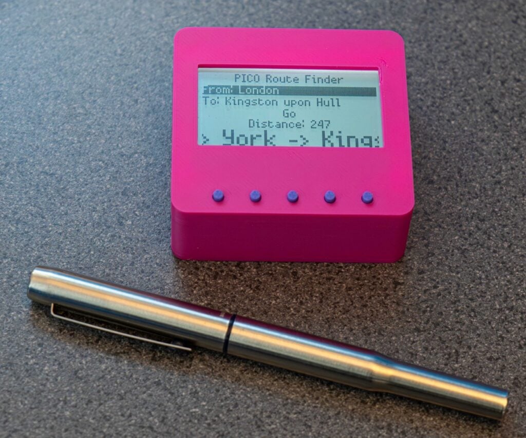
Figure 1 shows the Pico Route Finder. It contains map information for locations in the UK and will tell you the distance and the routes between them. Let’s look at how Dijkstra’s algorithm makes it work, starting with how the algorithm came about.

The story is that Dijkstra was having a coffee in Amsterdam and thinking about navigation. In the back of his mind, he was also wondering what he could write to demonstrate a new computer he was working on. After a few minutes of pondering, he came up with his algorithm, which boils down to three rules:

1. Keep track of how much it costs to go to places
2. Always use the lowest-cost route first when exploring
3. Keep track of where you have been

Let’s see how we can use these rules to find the cheapest route to some treasure. Suppose we are visiting a castle, and the owner tells us:

“I want you to chart a path from the Hall to my Treasure Room, where I have placed a pile of gold coins. You can have all the coins in the Treasure Room minus the cost of getting there. Each door on your path has a cost. You can roam the castle as much as you like, but when you have finished you can meet me in the Treasure Room, tell me the path you have devised, and I’ll give you your reward.”

Scores on the doors

We look around the Hall and see three labelled doors, as shown in Figure 2. The labels say ‘Kitchen: Cost 5’, ‘Library: Cost 2’, ‘Treasure Room: Cost 100’. We could go straight to the Treasure Room, which would cost us 100 coins. Or we could try our luck at finding a cheaper route. Fortunately, we are computer scientists familiar with Dijkstra’s algorithm, so we open our notebook and draw a table. Each door tells us about a new room and the cost of getting there from that room. We enter this information into our table, starting with the Hall, which is where we are now.

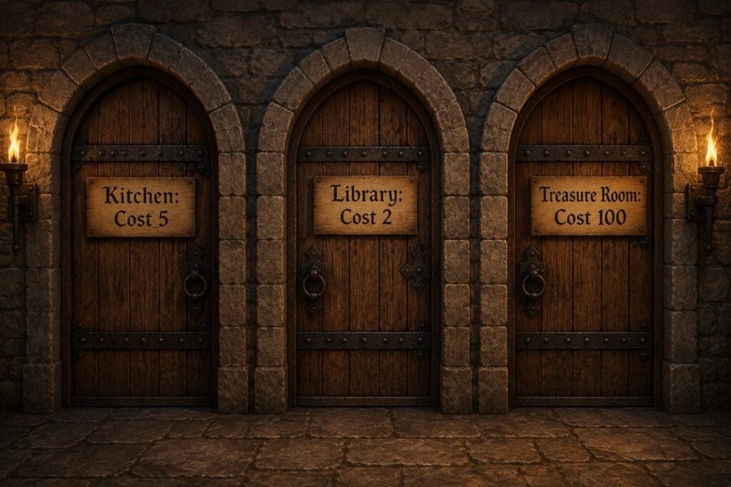
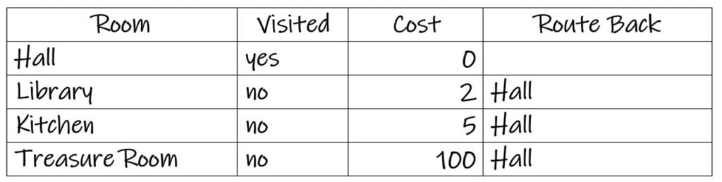
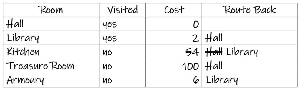
Figure 3 shows our first table. It describes rooms we know about, whether we have visited them, the cost of getting to each room from the Hall, and the route back to the start of our journey. Dijkstra’s algorithm says that we should now find the lowest-cost unvisited room, travel to that room, and update our table. So, we go to the Library. 

Want gold, will travel

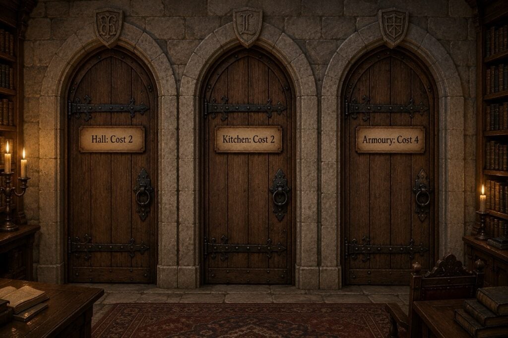
The doors in Figure 4 tell us it costs 2 to reach the Kitchen from the Library and 4 to reach the Armoury. They also tell us that it costs 2 to reach the Hall, but we already knew that from the door in the Hall. We use these numbers to update the table. Let’s start with the Armoury. It costs us 4 to get to the Armoury from the Library, and it costs 2 to get to the Library from the Hall. So, the total cost of getting to the Armoury from the Hall is 6. We add the Armoury to our table and note that the route back to the Hall from the Armoury starts by going to the Library and then going on to the Hall. 

Now we can update our table to save us some gold. Dijkstra’s algorithm tells us to keep track of journey costs. If we find a new cost that is less than one in the table, we need to update the table. It cost us 2 to get to the Library and it would cost 2 more to get from the Library to the Kitchen, making a total of 4. The cost of going directly from the Hall to the Kitchen was initially entered as 5 (the cost on the door in the Hall). But if we travel from the Hall to the Kitchen via the Library, we can save a gold coin. We update the table with this new information.

Figure 5 shows our updated table with out-of-date information crossed out. Our next stop will be the unvisited room with the lowest cost, which is the Kitchen. We go into the Kitchen and repeat this process until we end up in the Treasure room. 

The final reckoning

Figure 6 shows the table created during our travels. It tells us all we need to know. The cheapest route from the Hall to the Treasure Room costs 18 coins. We use the Route Back column in the table to find the way back from the Treasure Room to the Hall. The first step on the way back to the Hall is to visit the Bedroom. Then we look up the Route Back value for Bedroom to find the next step, and so on. The complete route back is Bedroom > Dining Hall > Kitchen > Library > Hall. You can work through this in Figure 6. We reverse this path to create a route from the Hall to the Treasure Room. 

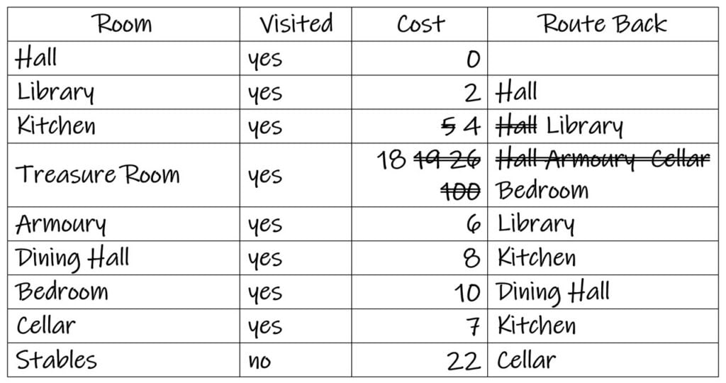
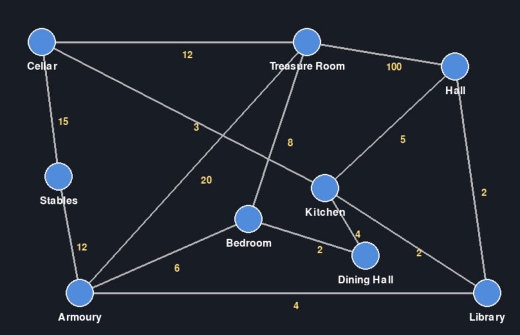
Figure 7 shows the map of the castle that we built on our travels. This is not complete. It only shows the rooms that we know about. If you want to prove that the algorithm works, you can work through the route-finding process to build the table shown in Figure 6.

Winning with Dijkstra 

The cleverness of the algorithm shines through when you notice how it has ignored places that are not on the best route. We never visited the Stables because routes there were more expensive than cheaper routes that we checked first. At the time Dijkstra came up with his theorem, computers had very limited main memory. His route-finding demonstration was limited to 64 locations because his program used six data bits to hold each location number. A huge part of Dijkstra’s initial triumph was fitting all the location information and the code into a very small amount of memory. 

Writing Dijkstra 

Rather than using a notebook to track costs, we can create our own cost-tracking program in Python. The first thing we need to do is create something to store each room:

class NodeRouteData:

def __init__(self, name, cost, route_back):

        self.name = name

        self.visited = False

        self.cost = cost

        self.route_back = route_back

The code above creates a class called NodeRouteData. This stores all the information about a location in the castle. We’re calling each location a ‘node’ because we might want to use this program to navigate things other than rooms in a castle. The class contains fields which map directly onto what we put in our notebook. When we create an instance of the class, we set the name, cost, and the route back from this node. Now let’s ask the user where they are starting from and where they are going:

start_name = input("Start name: ")

end_name = input("End name: ")

The statements above read the names of the start and end points and store them in variables called start_name and
end_name. Next, we need to make a node to represent the start location. We don’t need to make a node for the end location; we use the value in end_name to detect when we have found a route to it. 

start_node = NodeRouteData(start_name, 0, None)

The statement above creates a NodeRouteData called start_node, with the name set to start_name. The first argument to the constructor of NodeRouteData is the name of the node. The second argument is the cost of going there. For the start node this is 0, because it is where we start. The third argument is the route back (i.e. the place we go to on the way back to the start). Since this is the start, we have no route back, so this value is set to None. Now we need to put the start node in the table. We can use a Python dictionary to hold the table, and the name of a node will be used as the key to find that node in the dictionary.

nodes = {}

nodes[start_name] = start_node

The statements above create an empty dictionary called nodes and add the start room to it. You add an item to a dictionary by specifying a key (the thing that will be used to find the item), as shown above. Now we can start checking the doors in nodes and updating costs. We use a variable called current_node to refer to the node we are working on. At the start of our exploration, the current node will be the start node:

current_node = start_node

The statement above creates current_node and sets it to start_node. Now let’s kick off our loop:

while current_node.name != end_name:

The statement above starts a while loop that will cause the program to inspect nodes until it reaches one with the same name as the end of our route. Because the algorithm always chooses routes with the lowest cost, we will have found our cheapest route when the two names match. Inside the loop, we will do exactly what we did when we were physically exploring the castle. We look for doors and use the information on them to update our table. There might be more than one door, so we need to create a ‘door reading’ loop:

while True:

    name = input("Room name (empty to end): ")

    if name=="":

        break

The statements above create a loop that starts by asking for the name of a room from a door. If the name is an empty string, there are no more doors at this location, so the code uses a break to leave the door-reading loop. If the user has entered a name, the program asks for the cost of the route. 

cost_string = input("Cost :")

cost = int(cost_string)

The statements above set the variable cost_string to the string that the user types in and then convert this string into an integer stored in the variable cost. Now we can use this new cost value to update our table. The first thing we do is work out the cost of getting to the room on the door from the start location. This will be the cost of getting to this room, plus the cost on the door:

total_cost = cost + current_node.cost

We now have the name of a node and the total cost of getting to that node. If this is a node we haven’t seen before, we need to add it to the nodes. Let’s do that.

if name not in nodes:

    nodes[name]=NodeRouteData(name,
total_cost,current_node)

The code above checks the nodes dictionary to see if it contains an entry for the node with the name that was typed in. If the answer is no, the program adds a new node to the dictionary. We set the route back and the cost values for the new node. 

If the node is already in the dictionary, we need to check whether we have found a cheaper route to it. We can do this by adding an else part to the condition we just wrote. This code will run if the dictionary contains a node with the name on the door.

else:

    room=nodes[name]

    if total_cost < room.cost:

        room.cost = total_cost

        room.route_back = current_node

The code here gets a reference to the room from the dictionary and then compares the cost of using the newly discovered door with the stored cost of getting to that room. If the new route is cheaper, we update the room data. This is the programming equivalent of crossing out the cost and route-back entries in our notebook and writing new ones. 

Once all the door info from a room is known, the user will enter an empty room name and the room loop will end. Now we need to record that we’ve visited this room so we won’t go there again:

current_node.visited=True

Now that we have updated the route table, we need to decide where to go next. We need to find the next cheapest route in the table and go where that leads:

cheapest_node = None

for node in nodes.values():

    if node.visited:

        continue

    if cheapest_node == None or node.cost  < cheapest_node.cost:

        cheapest_node=node

This code sets the value of cheapest_node to the node which has not been visited and has the lowest cost. Now we can switch to it:

print(f"The next node is {cheapest_node.name}")

current_node = cheapest_node

These two statements tell the user where to go next and then set the value of current_node to the cheapest one. Note that the next node might not be through one of the doors that have just been discovered. At some point the loop will stop, because the cheapest_node becomes the one with the end name and the while loop will exit. This is where we tell the user the cost of the route and describe it to them. Displaying the cost of the route is the simpler of the two:

print(f"Cost: {current_node.cost}")

The search loop stops when the current_node refers to the node with the name of the end_node. So we just print out the cost of getting to the current node. This will print a cost of 18 coins. Now we build a route by working through all the route_back values of nodes in the route:

route = []

while current_node != None:

    route.append(current_node.name)

    current_node = current_node.route_back

The code above uses a loop to build a list called route. It starts at the end node and works back to the start. The start_node was created with a route_back value of None, so the loop will stop when it reaches the start. The loop adds the name of each node to the route list.

We now have a list of node names, but they are in the wrong order. We need to reverse them before printing them. 

route.reverse()

print("Route:", " -> ".join(route))

The two statements here reverse the route and then print out the names in the route, separated by ‘ -> ‘ strings. The rather wonderful join method works on a string, takes the elements in a collection, and inserts the string between each item in the collection. 

Hall -> Library -> Kitchen -> Dining Hall -> Bedroom -> Treasure Room

The statement above is the result of a successful run. The sample code for this article contains an implementation of the algorithm. If you’ve got this far, you are allowed to take a deep breath and feel very pleased with yourself. You now know how to implement Dijkstra’s algorithm. You also know more about Python classes, dictionaries, and references.

Map navigation

We can modify the castle navigation program to plot routes in the UK. First, we need a graph that describes routes between various locations. The word graph is used in lots of different contexts. The most familiar one is probably the Cartesian graph, which plots one value against another (for example, price against time). For routing, we use a node graph. This describes places (nodes) and routes between them. Here is one expressed as a JSON file.

The code in the map_graph.json listing shows the first part of the graph. It contains a dictionary of cities indexed by name. Cities have a geographical location and a list of links and costs (distances) to neighbouring cities. A modified version of the castle navigation program uses this node graph to find the shortest route between two cities. The Pico Route Finder uses the same code to create routes and then display them on the LCD panel.

Dijkstra forever

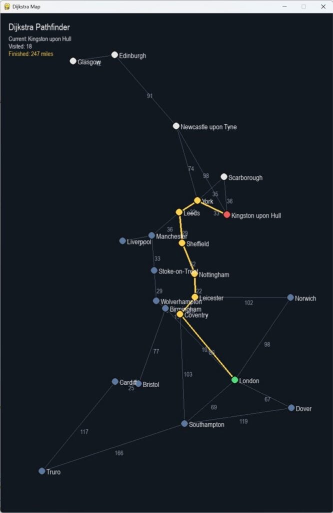
Dijkstra’s algorithm works by finding all the lowest-cost routes in order and stopping when it finds the required destination. When navigating from London to Hull, it found a route to Truro (a long way away from both London and Hull) before it found the route to Hull. For this reason, pure Dijkstra is not used in modern navigation, which tries to reduce the amount of route searching by making a judgement on whether a proposed route is moving towards or away from the destination. But there are many occasions where it is still the best way to create a route, and it will always be part of how computer systems find their way around.